参考

正文

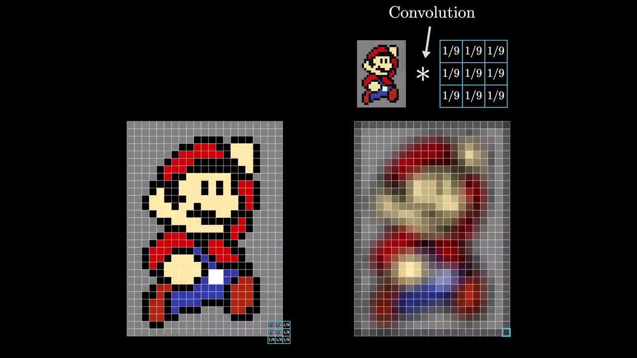
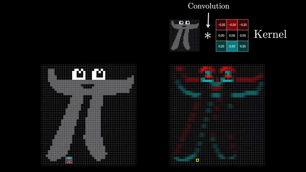
卷积运算

连续卷积：

$(f*g)(t):=\int_{-\infty}^{+\infty} f(x)\cdot g(t-x)dx$

离散卷积：

$\sum_{m=-M}^{M} f[n-m]g[m]$

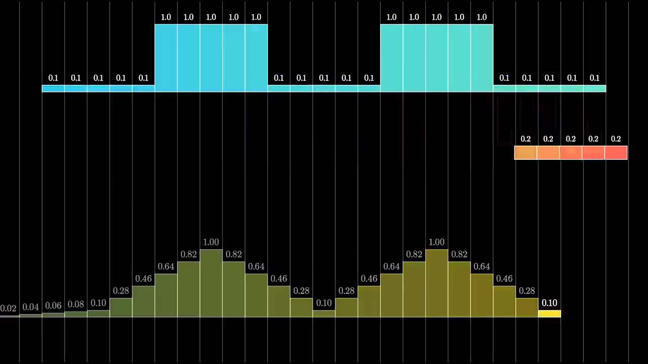
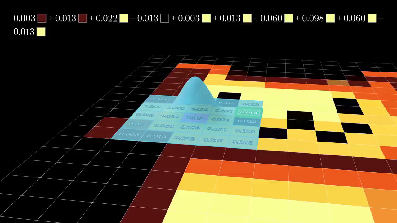
点对点相乘，再相加

使相乘后的数据拥有周边数据的一些特征：

在数字图像处理中的应用

import cv2
import matplotlib.pyplot as plt
import numpy as np

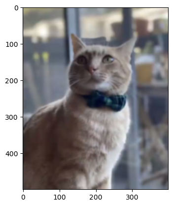
img = cv2.imread('images/tom_in_bowtie.jpg')
plt.imshow(cv2.cvtColor(img, cv2.COLOR_BGR2RGB))

<matplotlib.image.AxesImage at 0x2a11b90d760>

1	`img.shape`

(500, 399, 3)

def plot(array):
    print(array)
    plt.matshow(array, cmap='Wistia')
    plt.colorbar()
    for x in range(len(array)):
        for y in range(len(array)):
            plt.annotate(round(array[x, y], 3),xy=(x,y),horizontalalignment='center',
                         verticalalignment='center')
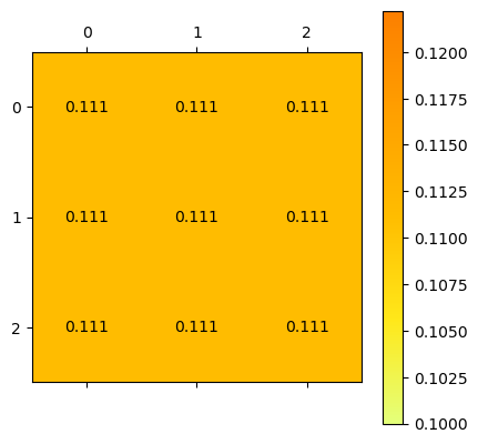
    return plt

均值滤波

1 2	`kernel = np.ones((3, 3)) / 9 plot(kernel)`

[[0.11111111 0.11111111 0.11111111]
 [0.11111111 0.11111111 0.11111111]
 [0.11111111 0.11111111 0.11111111]]



<module 'matplotlib.pyplot' from 'C:\\Users\\gzjzx\\anaconda3\\lib\\site-packages\\matplotlib\\pyplot.py'>

1 2	`fimg = cv2.filter2D(img, cv2.CV_8UC3, kernel) plt.imshow(cv2.cvtColor(fimg, cv2.COLOR_BGR2RGB))`

<matplotlib.image.AxesImage at 0x2a11c0d0af0>

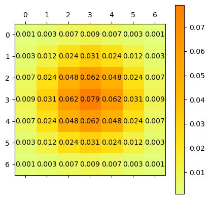
高斯模糊

定义高斯卷积核， $\sigma$ 为标准差

$G(x,y)=\frac{1}{2\pi\sigma^2}\exp\left(-\frac{x^2+y^2}{2\sigma^2}\right)$

或

$G(x,y)=\frac{1}{2\pi\sigma_x\sigma_y}\exp\left[-\left(\frac{x^2}{2\sigma^2_x}+\frac{y^2}{2\sigma^2_y}\right)\right]=\frac{1}{\sqrt{2\pi}\sigma_x}\exp\left(-\frac{x^2}{2\sigma^2_x}\right)\cdot \frac{1}{\sqrt{2\pi}\sigma_y}\exp\left(-\frac{y^2}{2\sigma^2_y}\right)=G(x)\cdot G(y)$

OpenCV2.4.13 源码分析-getGaussianKernel
@: python 中定义的矩阵乘法运算符

1 2	`def gaussian_kernel_2d(ksize, sigma): return cv2.getGaussianKernel(ksize, sigma) @ cv2.getGaussianKernel(ksize,sigma).T`

1 2	`kernel = gaussian_kernel_2d(7, -1) plot(kernel)`

[[0.00097656 0.00341797 0.00683594 0.00878906 0.00683594 0.00341797
  0.00097656]
 [0.00341797 0.01196289 0.02392578 0.03076172 0.02392578 0.01196289
  0.00341797]
 [0.00683594 0.02392578 0.04785156 0.06152344 0.04785156 0.02392578
  0.00683594]
 [0.00878906 0.03076172 0.06152344 0.07910156 0.06152344 0.03076172
  0.00878906]
 [0.00683594 0.02392578 0.04785156 0.06152344 0.04785156 0.02392578
  0.00683594]
 [0.00341797 0.01196289 0.02392578 0.03076172 0.02392578 0.01196289
  0.00341797]
 [0.00097656 0.00341797 0.00683594 0.00878906 0.00683594 0.00341797
  0.00097656]]



<module 'matplotlib.pyplot' from 'C:\\Users\\gzjzx\\anaconda3\\lib\\site-packages\\matplotlib\\pyplot.py'>

1	`sum(sum(kernel))`

1.0

应用高斯滤波

1 2	`fimg = cv2.filter2D(img, cv2.CV_8UC3, kernel) plt.imshow(cv2.cvtColor(fimg, cv2.COLOR_BGR2RGB))`

<matplotlib.image.AxesImage at 0x1c2abcbef70>

等效于

1 2	`fimg = cv2.GaussianBlur(img, (7, 7), -1) plt.imshow(cv2.cvtColor(fimg, cv2.COLOR_BGR2RGB))`

<matplotlib.image.AxesImage at 0x1c2aa6a6910>

锐化

kernel = np.array([[-0.5, -1.0, -0.5],
                   [-1.0, 7.0, -1.0],
                   [-0.5, -1.0, -0.5]])
plot(kernel)

[[-0.5 -1.  -0.5]
 [-1.   7.  -1. ]
 [-0.5 -1.  -0.5]]
0 0 -0.5
0 1 -1.0
0 2 -0.5
1 0 -1.0
1 1 7.0
1 2 -1.0
2 0 -0.5
2 1 -1.0
2 2 -0.5



<module 'matplotlib.pyplot' from 'C:\\Users\\gzjzx\\anaconda3\\lib\\site-packages\\matplotlib\\pyplot.py'>

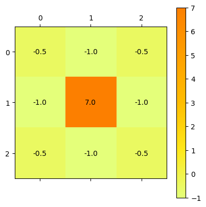
1	`sum(sum(kernel))`

1.0

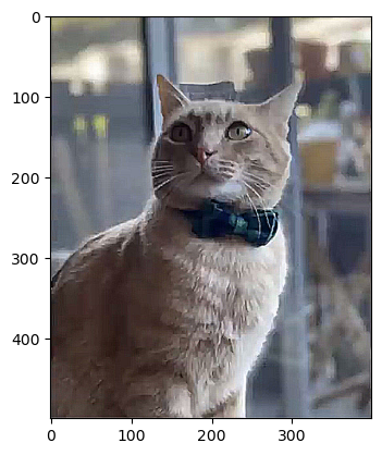
1 2	`fimg = cv2.filter2D(img, cv2.CV_8UC3, kernel) plt.imshow(cv2.cvtColor(fimg, cv2.COLOR_BGR2RGB))`

<matplotlib.image.AxesImage at 0x1c2a9376fd0>

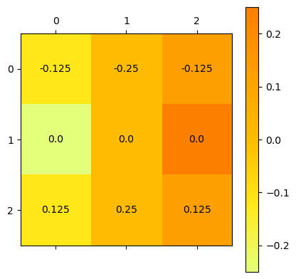
边缘检测

# 我也不知道这里为什么第二行显示的都是 0.0...
kernel = np.array([[-0.125, 0.0, 0.125],
                   [-0.25, 0.0, 0.25],
                   [-0.125, 0.0, 0.125]])
plot(kernel)

[[-0.125  0.     0.125]
 [-0.25   0.     0.25 ]
 [-0.125  0.     0.125]]



<module 'matplotlib.pyplot' from 'C:\\Users\\gzjzx\\anaconda3\\lib\\site-packages\\matplotlib\\pyplot.py'>

1	`sum(sum(kernel))`

0.0

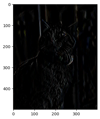
1 2	`fimg = cv2.filter2D(img, cv2.CV_8UC3, kernel) plt.imshow(4 * cv2.cvtColor(fimg, cv2.COLOR_BGR2RGB)) # 太黑了，我乘个 4`

<matplotlib.image.AxesImage at 0x2a11c124520>

Convolution via Fourier transform is faster

就是说卷积运算使用了太多的乘法，运用 FFT 算法的思想会加速运算？

import numpy as np

arr1 = np.random.random(100000)
arr2 = np.random.random(100000)

1 2	`%%timeit np.convolve(arr1, arr2)`

1.66s ± 341ms per loop (mean ± std. dev. of 7 runs, 1 loop each)

1	`import scipy.signal`

1 2	`%%timeit scipy.signal.fftconvolve(arr1, arr2)`

10.8ms ± 1.24ms per loop (mean ± std. dev. of 7 runs, 100 loops each)

定义法

def conv(a, b):
    N = len(a)
    M = len(b)
    YN = N + M - 1
    y = [0.0 for i in range(YN)]
    for n in range(YN):
        for m in range(M):
            if 0 <= n - m and n - m < N:
                y[n] += a[n - m] * b[m]
    return y

1	`conv((1, 2, 3), (4, 5, 6))`

[4.0, 13.0, 28.0, 27.0, 18.0]

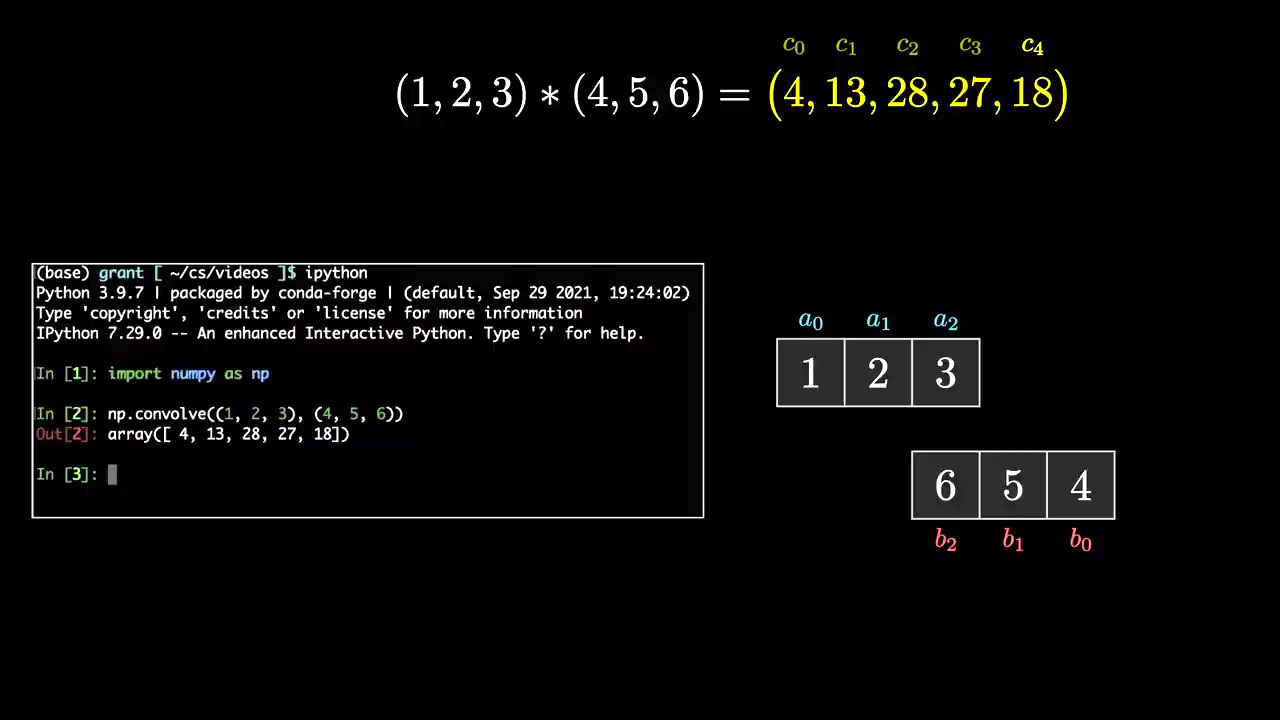
使用 numpy 库

1
2
3

import numpy as np

np.convolve((1, 2, 3), (4, 5, 6))

array([ 4, 13, 28, 27, 18])

FFT 快速卷积

def convfft(a, b):
    N = len(a)
    M = len(b)
    YN = N + M - 1
    FFT_N = 2 ** (int(np.log2(YN)) + 1)
    afft = np.fft.fft(a, FFT_N)
    bfft = np.fft.fft(b, FFT_N)
    abfft = afft * bfft
    y = np.fft.ifft(abfft).real[:YN]
    return y

1	`convfft((1, 2, 3), (4, 5, 6))`

array([ 4., 13., 28., 27., 18.])

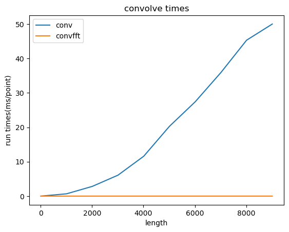
对比

import time
import matplotlib.pyplot as plt

def run(func, a, b):
    n = 1
    start = time.perf_counter()
    for j in range(n):
        func(a, b)
    end = time.perf_counter()
    run_time = end - start
    return run_time / n

n_list = []
t1_list = []
t2_list = []
for i in range(10):
    count = i * 1000 + 10
    print(count)
    a = np.ones(count)
    b = np.ones(count)
    t1 = run(conv, a, b)  # 直接卷积
    t2 = run(convfft, a, b)  # FFT 卷积
    n_list.append(count)
    t1_list.append(t1)
    t2_list.append(t2)

# plot
plt.plot(n_list, t1_list, label='conv')
plt.plot(n_list, t2_list, label='convfft')
plt.legend()
plt.title(u"convolve times")
plt.ylabel(u"run times(ms/point)")
plt.xlabel(u"length")
plt.show()