官网
课程
3 如何选择机器学习方法
流程图
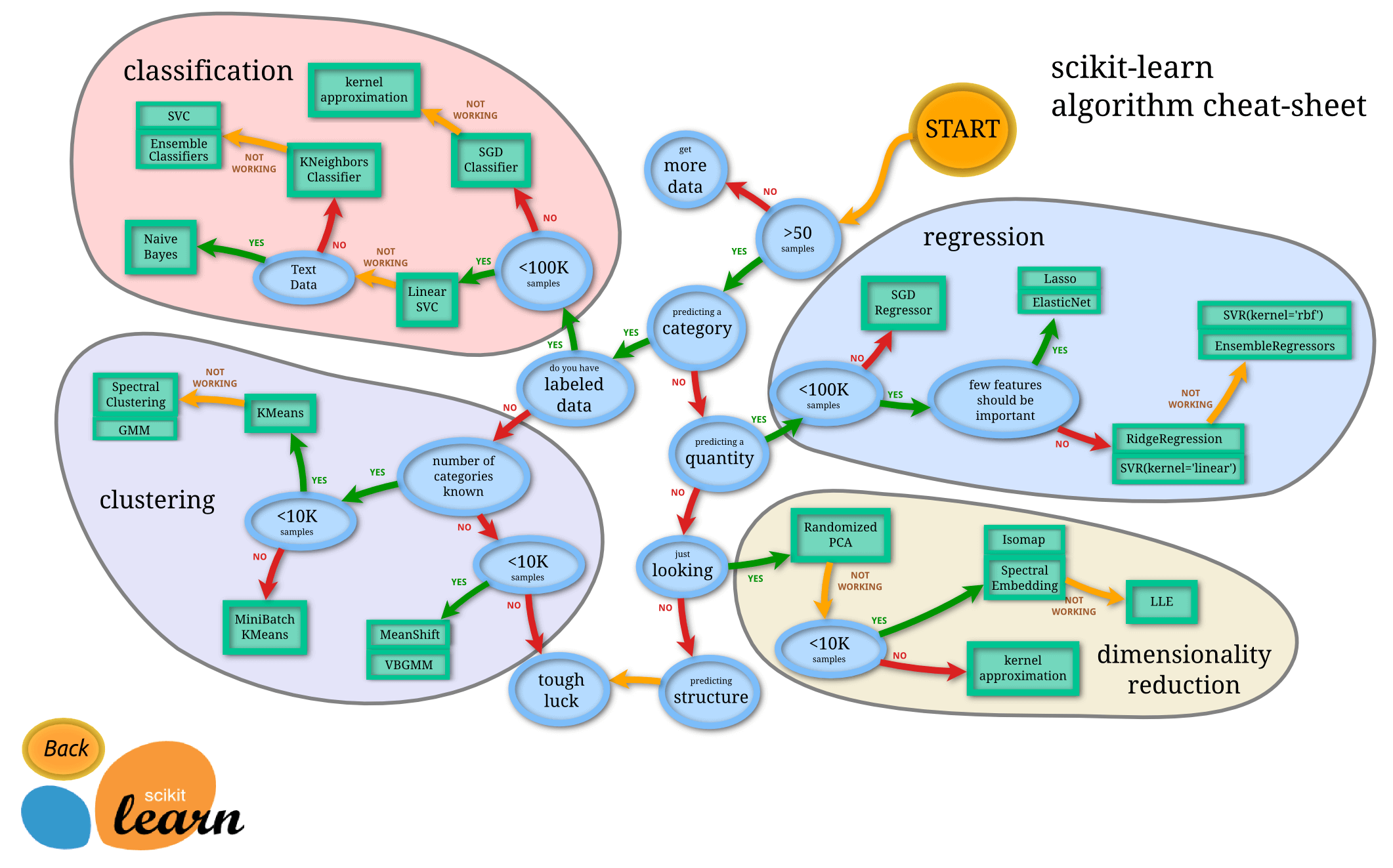
-
classification 分类
-
regression 回归
-
clustering 聚类
-
dimensionality reduction 数据降维
4 通用学习模式
导入数据集
查看 iris 的属性:
import numpy as np
from sklearn import datasets
from sklearn.model_selection import train_test_split  # from sklearn.cross_validation import train_test_split
from sklearn.neighbors import KNeighborsClassifier  # KNN K 临近算法

iris = datasets.load_iris()
iris_X = iris.data
iris_y = iris.target

iris_X[:2, :]
array([[5.1, 3.5, 1.4, 0.2],
[4.9, 3. , 1.4, 0.2]])
查看 iris 的分类结果:
iris_yarray([0, 0, 0, 0, 0, 0, 0, 0, 0, 0, 0, 0, 0, 0, 0, 0, 0, 0, 0, 0, 0, 0,
0, 0, 0, 0, 0, 0, 0, 0, 0, 0, 0, 0, 0, 0, 0, 0, 0, 0, 0, 0, 0, 0,
0, 0, 0, 0, 0, 0, 1, 1, 1, 1, 1, 1, 1, 1, 1, 1, 1, 1, 1, 1, 1, 1,
1, 1, 1, 1, 1, 1, 1, 1, 1, 1, 1, 1, 1, 1, 1, 1, 1, 1, 1, 1, 1, 1,
1, 1, 1, 1, 1, 1, 1, 1, 1, 1, 1, 1, 2, 2, 2, 2, 2, 2, 2, 2, 2, 2,
2, 2, 2, 2, 2, 2, 2, 2, 2, 2, 2, 2, 2, 2, 2, 2, 2, 2, 2, 2, 2, 2,
2, 2, 2, 2, 2, 2, 2, 2, 2, 2, 2, 2, 2, 2, 2, 2, 2, 2])
train_test_split 分离数据集(测试集/训练集):
# 测试集 : 训练集 = 7 : 3
X_train, X_test, y_train, y_test = train_test_split(iris_X, iris_y, test_size=0.3)
y_train
array([1, 0, 2, 2, 2, 0, 2, 2, 2, 1, 1, 0, 0, 0, 0, 0, 0, 2, 0, 1, 0, 2,
0, 0, 1, 0, 0, 1, 1, 2, 0, 1, 2, 2, 2, 2, 2, 2, 1, 2, 0, 0, 2, 2,
0, 1, 1, 2, 2, 2, 2, 0, 0, 2, 1, 1, 1, 2, 2, 1, 0, 2, 1, 2, 0, 0,
1, 0, 2, 1, 2, 0, 1, 2, 1, 2, 1, 0, 0, 1, 1, 2, 2, 1, 0, 2, 1, 1,
0, 0, 1, 1, 1, 2, 0, 0, 2, 1, 2, 2, 1, 2, 1, 2, 2])
使用 KNN 算法进行分类
knn = KNeighborsClassifier()
# fit 训练
knn.fit(X_train, y_train)
# predict 生成预测结果
knn.predict(X_test)
array([2, 2, 0, 2, 1, 1, 1, 1, 1, 0, 0, 2, 0, 2, 1, 2, 0, 2, 2, 0, 1, 1,
1, 0, 0, 1, 1, 0, 2, 0, 1, 2, 0, 1, 2, 1, 0, 0, 2, 0, 0, 0, 0, 0,
1])
y_testarray([1, 2, 0, 2, 1, 1, 1, 1, 1, 0, 0, 2, 0, 2, 1, 1, 0, 2, 2, 0, 1, 1,
1, 0, 0, 1, 1, 0, 1, 0, 1, 2, 0, 1, 2, 1, 0, 0, 2, 0, 0, 0, 0, 0,
1])
看出预测结果与 y_test 基本相似
5sklearn 的 datasets 数据库
from sklearn import datasets
from sklearn.linear_model import LinearRegression  # 线性回归

loaded_data = datasets.load_boston()  # 波士顿房价数据库
data_X = loaded_data.data
data_y = loaded_data.target

model = LinearRegression()
model.fit(data_X, data_y)

model.predict(data_X[:4, :])

# 这里原作者忘记分割数据集了..
array([30.00384338, 25.02556238, 30.56759672, 28.60703649])
data_y[:4]array([24. , 21.6, 34.7, 33.4])
创造数据库
import matplotlib.pyplot as plt

plt.figure()
X, y = datasets.make_regression(n_samples=100, n_features=1, n_targets=1, noise=10)
plt.scatter(X, y)
plt.show()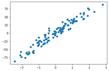
6model 常用属性和功能
from sklearn import datasets
from sklearn.linear_model import LinearRegression  # 线性回归

loaded_data = datasets.load_boston()  # 波士顿房价数据库
data_X = loaded_data.data
data_y = loaded_data.target

model = LinearRegression()
model.fit(data_X, data_y)
model.coef_ 斜率
在 fit 之后输出的 coef和 intercept才会比较准确
model.coef_ # 各个属性对应的斜率array([-1.08011358e-01, 4.64204584e-02, 2.05586264e-02, 2.68673382e+00,
-1.77666112e+01, 3.80986521e+00, 6.92224640e-04, -1.47556685e+00,
3.06049479e-01, -1.23345939e-02, -9.52747232e-01, 9.31168327e-03,
-5.24758378e-01])
model.intercept_ 截距
model.intercept_ # 截距(与 Y 轴的交点)36.45948838509036
model.get_params() 查看定义的参数
model.get_params(){'copy_X': True,
'fit_intercept': True,
'n_jobs': None,
'normalize': 'deprecated',
'positive': False}
model.score() 对 model 学到的东西进行打分
model.score(data_X, data_y) # 确定性系数 R^2, 将预测结果与实际结果进行分析, 看吻合程度0.7406426641094095
7 normalization 标准化数据
preprocessing.scale()
from sklearn import preprocessing  # 预处理
import numpy as np

a = np.array([[10, 2.7, 3.6],
              [-100, 5, -2],
              [120, 20, 40]], dtype=np.float64)
# 每个列代表一个属性
# 属性 1 取值范围: [-100, 120]
# 属性 2 取值范围: [2.7, 20]
# 属性 3 取值范围: [-2, 40]
# 各个属性取值范围差距较大
preprocessing.scale(a)
array([[ 0. , -0.85170713, -0.55138018],
[-1.22474487, -0.55187146, -0.852133 ],
[ 1.22474487, 1.40357859, 1.40351318]])
经过标准化处理后, 各个属性取值范围基本一致
实例
from sklearn import preprocessing  # 预处理
import numpy as np
from sklearn.model_selection import train_test_split  # 分割数据集
from sklearn.datasets import make_classification  # 创建数据
from sklearn.svm import SVC  # Support Vector classifier 支持向量分类器
import matplotlib.pyplot as plt  # 可视化

X, y = make_classification(n_samples=300, n_features=2, n_redundant=0, n_informative=2,
                          random_state=22, n_clusters_per_class=1, scale=100)
plt.figure()
plt.scatter(X[:, 0], X[:, 1], c=y)  # c=y: color=yellow
plt.show()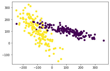
X, y = make_classification(n_samples=300, n_features=2, n_redundant=0, n_informative=2,
                          random_state=22, n_clusters_per_class=1, scale=1000)
X = preprocessing.scale(X)
X_train, X_test, y_train, y_test = train_test_split(X, y, test_size=.3)
clf = SVC()
clf.fit(X_train, y_train)
# 用 training data 学习, 用 test data 去预测
clf.score(X_test, y_test)
0.9222222222222223
8 cross validation 交叉验证 1
常规
from sklearn.datasets import load_iris
from sklearn.model_selection import train_test_split
from sklearn.neighbors import KNeighborsClassifier

iris = load_iris()
X = iris.data
y = iris.target

X_train, X_test, y_train, y_test = train_test_split(X, y, random_state=4)
knn = KNeighborsClassifier(n_neighbors=5)  # 考虑数据附近的 5 给 neighbor
knn.fit(X_train, y_train)
y_pred = knn.predict(X_test)
knn.score(X_test, y_test)
0.9736842105263158
交叉验证
from sklearn.datasets import load_iris
from sklearn.model_selection import train_test_split
from sklearn.neighbors import KNeighborsClassifier

iris = load_iris()
X = iris.data
y = iris.target

from sklearn.model_selection import cross_val_score
knn = KNeighborsClassifier(n_neighbors=5)  # 考虑数据附近的 5 给 neighbor
scores = cross_val_score(knn, X, y, cv=5, scoring="accuracy")  # 判断其准确度是否够高
scores
array([0.96666667, 1. , 0.93333333, 0.96666667, 1. ])
scores.mean() # 平均结果0.9733333333333334
判断如何选择参数取值最佳
看精确度
from sklearn.model_selection import cross_val_score
import matplotlib.pyplot as plt

k_range = range(1, 31)
k_scores = []
for k in k_range:
    knn = KNeighborsClassifier(n_neighbors=k)
    scores = cross_val_score(knn, X, y, cv=10, scoring="accuracy")
    k_scores.append(scores.mean())
plt.figure()
plt.plot(k_range, k_scores)
plt.xlabel("Value of K for KNN")
plt.ylabel('Cross-Validated Acuracy')
plt.show()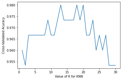
- 如果 K 过小, 会出现欠拟合问题
- 如果 K 过大, 会出现 overfitting 问题(过拟合)
9 cross validation 交叉验证 2
过拟合问题
from sklearn.model_selection import learning_curve  # 可视化训练的过程
from sklearn.datasets import load_digits
from sklearn.svm import SVC
import matplotlib.pyplot as plt
import numpy as np

digits = load_digits()
X = digits.data
y = digits.target
train_sizes, train_loss, test_loss = learning_curve(
    SVC(gamma=0.01), X, y, cv=10, scoring='neg_mean_squared_error',
    train_sizes=[0.1, 0.25, 0.5, 0.75, 1])
train_loss_mean = -np.mean(train_loss, axis=1)
test_loss_mean = -np.mean(test_loss, axis=1)

plt.figure()
plt.plot(train_sizes, train_loss_mean, 'o-', color='r', label='Training')
plt.plot(train_sizes, test_loss_mean, 'o-', color='g', label='Cross-validation')
plt.xlabel('Training examples')
plt.ylabel('Loss')
plt.legend(loc='best')
plt.show()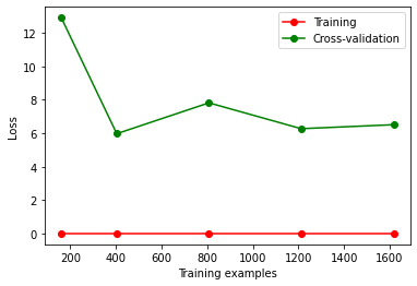
出现过拟合, 当样本数据量变大时误差率反而增加
10 cross validation 交叉验证 3
from sklearn.model_selection import validation_curve
from sklearn.datasets import load_digits
from sklearn.svm import SVC
import matplotlib.pyplot as plt
import numpy as np

digits = load_digits()
X = digits.data
y = digits.target
param_range = np.logspace(-6, -2.3, 5)
train_loss, test_loss = validation_curve(
    SVC(), X, y, param_name='gamma', param_range=param_range, cv=10,
    scoring='neg_mean_squared_error')
train_loss_mean = -np.mean(train_loss, axis=1)
test_loss_mean = -np.mean(test_loss, axis=1)

plt.figure()
plt.plot(param_range, train_loss_mean, 'o-', color='r', label='Training')
plt.plot(param_range, test_loss_mean, 'o-', color='g', label='Cross-validation')
plt.xlabel('gamma')
plt.ylabel('Loss')
plt.legend(loc='best')
plt.show()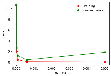
11 保存 model
from sklearn import svm
from sklearn import datasets

clf = svm.SVC()
iris = datasets.load_iris()
X, y = iris.data, iris.target
clf.fit(X, y)
SVC()
方法 1: pickle
导出
import pickle

with open('save/clf.pickle', 'wb') as f:
    pickle.dump(clf, f)
导入
with open('save/clf.pickle', 'rb') as f:
    clf2 = pickle.load(f)
clf2.predict(X[0:1])
array([0])
方法 2: joblib
导出
import joblib

joblib.dump(clf, 'save/clf.pkl')
['save/clf.pkl']
导入
clf3 = joblib.load('save/clf.pkl')
clf3.predict(X[0:1])
array([0])